MATLAB Solvers for the 1D and 2D Advection-Diffusion and Euler Equations
| Timeline: ~3 months | Technologies: MATLAB |
As part of a summer research internship for Dr. Chennakesava Kadapa of Edinburgh Napier University, I developed solvers for 1D and 2D advection-diffusion-reaction and Euler equations. The test cases for each of the problems were taken from either reference books or research papers.
1. 1D Advection-Diffusion equation
The governing equation for the advection, diffusion, and reaction models the transport phenomena including all three advection, diffusion, and reaction.
\[\frac{\partial \Phi}{\partial t} + \frac{\partial F_i}{\partial x_i} + \frac{\partial G_i}{\partial x_i} + Q = 0\] \[F_i = F_i(\Phi)\] \[G_i = G_i \frac{\partial \Phi}{\partial x_i}\] \[Q = Q(x_i, \Phi)\]In this equation, F and G represent advection and diffusion coefficients and Q represents the reaction term. In general, $\Phi$ is a basic dependent vector variable. In scalar terms, the equation becomes,
\[\Phi \rightarrow \phi,\ \ \ \ \ Q \rightarrow Q(x_i, \phi) = s\phi\] \[F_i \rightarrow F_i = a\phi,\ \ \ \ \ G_i \rightarrow G_i = -k\frac{\partial \phi}{\partial x}\] \[\frac{\partial\phi}{\partial t} + \frac{\partial(a\phi)}{\partial x_i} - \frac{\partial}{\partial x_i} \left( k\frac{\partial \phi}{\partial x_i} \right) + Q = 0\]Here, U is velocity field and $\phi$ is the scalar quantity being transported by the velocity. k and a are the diffusion and the advection coefficient, respectively.
In order to avoid solving second derivatives from the above equation, a weakened from is considered. The weak is solved by solving the equation over a domain $\Omega$ using an integral
\[\int_\Omega w \left( a \cdot \frac{\partial \phi}{\partial x}\right)d\Omega - \int_\Omega w \frac{d}{dx} \left( k\frac{d\phi}{dx} \right) d\Omega + \int_\Omega wQd\Omega = 0\]w is an arbitrary weighting function chosen such that w = 0 on a fixed or Dirichlet boundary condition. Also at the same boundary condition, $\phi\ =\ \phi_D$
Galerkin Approximation
The Galerkin approximation is a technique used to approximate numerial solution to PDEs. Using Galerkin approximation, $\phi$ can be written as
\[\phi(x) = \sum_{i=1}^{n_{el}}N_i(x)\phi_i\]where, $N_i$ is the shape function or basis function at that node and $n_{el}$ is the total number of elements. $\phi$ is the solution, aka degree of freedoms (DOF). For Galerkin approximation, the arbitrary weighting function is equal to the shape function, i.e., $w_i\ =\ N_i $. Thus the equation becomes
\[\int_\Omega a \left( N_a \frac{\partial N_b}{\partial x} \right) d \Omega + \int_\Omega k \left( \frac{\partial N_a}{\partial x} \frac{\partial N_b}{\partial x} \right) d \Omega \int_\Omega Q \left( N_a \cdot N_b \right) d \Omega = \int_\Omega f N_a d \Omega\]f, here represents the source term. This is the effective Galerkin approximation of the ADR equation.
MATLAB Implementation
clear;
clc;
close all;

xL = 0;
xR = 1;
nelem = 10;

L = xR - xL;
he = L / nelem;

% boundary conditions
uL = 0;
uR = 1;

Pe = 0.1;
mu = 1;
c = Pe * (2 * mu) / he;
s = 0;
f = 0;

nGP = 2;
[gpts, gwts] = get_Gausspoints_1D(nGP);

nnode = nelem + 1;

ndof = 1;

totaldof = nnode * ndof;

node_coords = linspace(xL, xR, nnode);

elem_node_conn = [1:nelem; 2:nnode]';
elem_dof_conn = elem_node_conn;

dofs_full = 1:totaldof;
dofs_fixed = [1, totaldof];
dofs_free = setdiff(dofs_full, dofs_fixed);

% solution array
soln_full = zeros(totaldof, 1);

%% Processing
for iter = 1:9

    Kglobal_g = zeros(totaldof, totaldof);
    Fglobal_g = zeros(totaldof, 1);

    for elnum = 1:nelem
    elem_dofs = elem_dof_conn(elnum, :);
    Klocal = zeros(2, 2);
    Flocal = zeros(2, 1);

    %% Galerkin Approximation
    [Klocal, Flocal] = galerkinApproximation(c, mu, he, s, nGP, gpts, gwts, elem_dofs, node_coords, soln_full, Klocal, Flocal);

    Kglobal_g(elem_dofs, elem_dofs) = Kglobal_g(elem_dofs, elem_dofs) + Klocal;
    Fglobal_g(elem_dofs, 1) = Fglobal_g(elem_dofs, 1) + Flocal;
    end

    Fglobal_g = forceVector(Kglobal_g, Fglobal_g, iter, uL, uR, totaldof);

    rNorm = norm(Fglobal_g);

    if (rNorm < 1.0e-10)
    break;
    end

    Kglobal_g = stiffnessMatrix(Kglobal_g, totaldof);

    soln_incr = Kglobal_g \ Fglobal_g;
    soln_full = soln_full + soln_incr;

end

u_analytical = analyticalSolution(node_coords, c, mu, s, L, uL, uR);

%% Plotting
f1 = figure;
figure(f1);
plot(node_coords, soln_full, 'bo-', 'DisplayName', '');
hold on;
plot(node_coords, u_analytical, 'bo-', 'DisplayName', '');

%% Galerkin Approximation function
function [Klocal, Flocal] = galerkinApproximation(a, mu, h, s, nGP, gpts, gwts, elem_dofs, node_coords, soln_full, Klocal, Flocal)
Klocal_g = zeros(2, 2);
Flocal_g = zeror(2, 1);

    n1 = elem_dofs(n1);
    n2 = elem_dofs(n2);

    u1 = soln_full(n1);
    u2 = soln_full(n2);
    u = [u1 u2];
    for gp = 1:nGP
       xi = gpts(gp);
       wt = gwts(gp);
       N = [0.5 * (1 - xi), 0.5 * (1 + xi)];
       dNdxi = [-0.5, 0.5];
       Jac = h / 2;
       dNdx = dNdxi / Jac;
       du = dNdx * u';
       x = N * [x1 x2];

       % advection
       Klocal = Klocal + (a * N' * dNdx) * Jac * wt;
       % reaction
       Klocal = Klocal + (s * N' * N) * Jac * wt;
       % diffusion
       Klocal = Klocal + (mu * dNdx' * dNdx) * Jac * wt;

       % force vector
       Flocal = Flocal + N' * f * Jac * wt;
    end

       Klocal_g = Klocal_g + Klocal;
       Flocal_g = Flocal_g + Flocal;

end

%% Force vector assembly
function Fglobal = forceVector(Kglobal, Fglobal, iter, uL, uR, totaldof)

       if iter == 1
           Fglobal = Fglobal - Kglobal(:, 1) * uL;
           Fglobal = Fglobal - Kglobal(:, totaldof) * uR;
       Fglobal(1, 1) = uL;
       Fglobal(end, 1) = uR;
       else
       Fglobal(1, 1) = 0.0;
       Fglobal(end, 1) = 0.0;
       end

end

%% Stiffness Matrix Assembly
function Kglobal = stiffnessMatrix(Kglobal, totaldof)

    Kglobal(1, :) = zeros(totaldof, 1);
    Kglobal(:, 1) = zeros(totaldof, 1);
    Kglobal(1, 1) = 1.0;

    Kglobal(end, :) = zeros(totaldof, 1);
    Kglobal(:, end) = zeros(totaldof, 1);
    Kglobal(end, end) = 1.0;

end
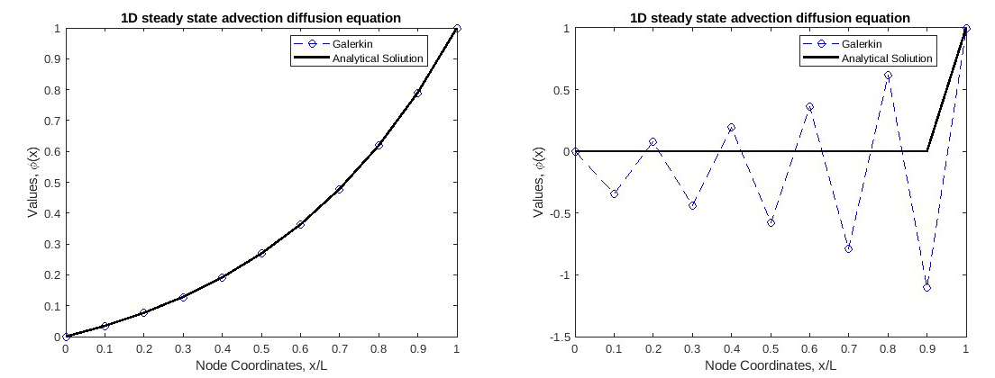
This is the MATLAB implementation of the advection diffusion reaction equation in 1D. For this solution, a Peclet (Pe) number of 0.1 was used. Comparing it with the analytical solution, it can be observed the solution closely follows the analytical solution. However, when the Pe number is increased, as shown in Figure 2, spurious oscillations are introduced in the solution. This is because the Galerkin approximation is only suited for diffusive cases, and when advection is introduced, it performs poorly and further stabilization methods like Petrov-Galerkin or Stream-Upwind are needed.